GAMMA Questions

Good question.
Are these bistatic Tandem or two-pass?
For my Colima (Spotlight) data the range std is usually < 0.1. The azimuth std varies a bit more, and tends to be slightly larger for baselines > 200 m, but usually still < 0.2. I compared two interferograms with
final model fit std. dev. (samples) range: 0.0346 azimuth: 0.0357
final model fit std. dev. (samples) range: 0.0925 azimuth: 0.2451
And they both look equally fine... would be interesting to hear other peoples thoughts here.

In this case it's two-pass TSX StripMap data. For some scenes I get easily values below 0.1, but for some I am really struggeling. In wonder if coregistration is than done also above the glaciated area, despite that I have set the SNR value quite high (I am playing around with values between 20.0 - 30.0). It may be possible that I have than a regular shift in my data? That would not be good, since I'd like to do offset tracking afterwards. Thus, precise coregistration is essential.

EDIT: The glaciated areas cover sometimes quite a big part of the image (distributed over the entire scene). So I guess, I am struggeling to build my routines in a way that coregistration is done only over the stable part.

So after lots of try and error, here is my ultimate solution:

I found out that the iteration of offset_fit can actually be managed manually. And this gives you absolute control over the precision of you coregistration.

Take now my example: two StripMap TSX scenes to be coregistered, whereas the master has a width of 14350 and a length of 18923 pixels.

You start with the usual create_offset and init_offset_orbit in order to get a first estimate.

Than you could follow on:

offset_pwr <SLC-1> <SLC-2> <SLC1_par> <SLC2_par> <OFF_par> <offs> <snr> 64 64 - 2 230 300 7.0 0
...
Result: number of offsets above SNR threshold: 16269 of 69000

I choose equal window sizes of 64, an oversampling of 2 and a large amount of windows in range and azimuth direction ( e.g 14350/64=~230), since I'd like to get many good values (they will be reduced in the following step). Also important: do not use a large SNR threshold here, you may want to keep these values, you can still sort out by SNR later on.

Now the clou: enable the interact_mode of offset_fit (last flag=1)!

offset_fit <offs> <snr> <OFF_par> [coffs] [coffsets] 7.0 4 1

Leave the threshold low in order to keep as much good values as possible. I used a polynomial with 4 parameters and enabled the interactive mode.
Now you see something like this

...
number of offset polynomial parameters: 4: a0 + a1*x + a2*y + a3*x*y
MODE: interactive culling of offsets
number of range samples: 230  number of azimuth samples: 300
number of samples in offset map: 69000
range sample spacing: 62  azimuth sample spacing: 62
solution: 16269 offset estimates accepted out of 69000 samples

range fit SVD singular values:        1.42470e+11   3.97305e+02   9.44447e+06   4.91438e+06
azimuth fit SVD singular values:      1.42470e+11   3.97305e+02   9.44447e+06   4.91438e+06
range offset poly. coeff.:               86.72567   1.14363e-03  -3.55814e-04   3.24785e-08
azimuth offset poly. coeff.:            -31.59035  -1.83796e-05  -9.41610e-05   3.48082e-09
model fit std. dev. (samples) range:  11.0689  azimuth:   5.3760

enter minimum SNR threshold:

You enter the minimum SNR threshold of the values you'd like to keep (e.g. 7.0).

enter the range and azimuth error thresholds:

Here you define the error thresholds. Looking at the values above (model fit std. dev. (samples) range: 11.0689 azimuth: 5.3760), I choose: 11 and 5

range, azimuth error thresholds:    11.0000     5.0000
SNR threshold:     7.0000

range fit SVD singular values:        9.39640e+10   3.25952e+02   8.06337e+06   3.22973e+06
azimuth fit SVD singular values:      9.39640e+10   3.25952e+02   8.06337e+06   3.22973e+06

*** improved least-squares polynomial coefficients 1 ***
solution: 12912 offset estimates accepted out of 69000 samples
range offset poly. coeff.:               81.81000   2.70354e-03  -4.08702e-04   2.24058e-08
azimuth offset poly. coeff.:            -31.87160   8.13869e-05  -8.37414e-05   4.51230e-11
model fit std. dev. (samples) range:   2.9335  azimuth:   0.9042

interate and further refine the offset fit? (1=yes, 0=no):

Now you see that a lot of points got rejected and the model fit parameters look much nicer. But of course, we are not satisfied yet, so we continue and use new error thresholds of e.g. 3 and 1:

range, azimuth error thresholds:     3.0000     1.0000
SNR threshold:     7.0000

range fit SVD singular values:        8.40150e+10   2.74138e+02   7.20409e+06   2.65694e+06
azimuth fit SVD singular values:      8.40150e+10   2.74138e+02   7.20409e+06   2.65694e+06

*** improved least-squares polynomial coefficients 1 ***
solution: 10018 offset estimates accepted out of 69000 samples
range offset poly. coeff.:               81.15585   2.97471e-03  -4.13961e-04   1.88112e-08
azimuth offset poly. coeff.:            -31.83394   8.21711e-05  -9.27860e-05   8.66807e-10
model fit std. dev. (samples) range:   1.4540  azimuth:   0.3338

interate and further refine the offset fit? (1=yes, 0=no):

And so on, until you are satisfied:

enter the range and azimuth error thresholds: 0.12 0.1
range, azimuth error thresholds:     0.1200     0.1000
SNR threshold:     7.0000

range fit SVD singular values:        1.70591e+10   4.32403e+01   1.39960e+06   3.20638e+05
azimuth fit SVD singular values:      1.70591e+10   4.32403e+01   1.39960e+06   3.20638e+05

*** improved least-squares polynomial coefficients 1 ***
solution: 438 offset estimates accepted out of 69000 samples
range offset poly. coeff.:               81.17558   3.08108e-03  -4.81343e-04   1.54942e-08
azimuth offset poly. coeff.:            -31.68129   5.27311e-05  -1.06932e-04   2.23491e-09
model fit std. dev. (samples) range:   0.0727  azimuth:   0.0420

It is really important that you carefully interate and do not set your desired threshold down to 0.1 from the beginning, otherwise you would use a lot of points, since the first bad fit is taken as a reference. You also need to be really careful when entering values. Unfortunately, you cannot correct wrong entries - one wrong button pressed and you can start from anew (really annoying).

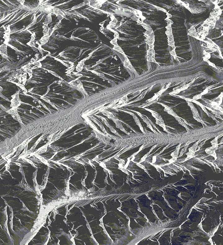
In my example we have 438 good points left. Now, lets have a look how they are actually distributed. A fit is only good, if the distribution is well over the entire image area. One possibility to get an impression is to plot the points on an image. We'd like to stick with GAMMA, since we do not want to step out of a batch... (no MATLAB here ;))

So first, generate an ras/bmp image of your MLI file (you can use the SLC file aswell, but that's incredibly huge and the power image is sufficient for our needs).

raspwr demo.mli 1435

Than we need to get our points that are used for the fitting. They are stored in the *.coffsets file and we can prepare them by using text2pt like the following. The first 0 says we want to have point list coordinates and the second 0 defines the starting column.

text2pt demo.coffsets 0 0 demo.pts

Than we want to overlay the points on our image:

ras_pt demo.pts - mli.bmp mli_points.bmp 10 12 255 255 255 15

10 and 12 are my multilooking values and the next 3 numbers set up the RGB colour you'd like to have for the crosses. 15 is the cross size. And this is what you get:

Nice overview, but of course I am not happy with the distribution of the points. I think I should incredibly reduce the number of windows from the beginning (during try and error I generated a better example). I could also have a look at the points that are located over glaciated area and have a look what kind of SNR they actually have (look in *.coffsets file). I may than increase my SNR threshold a bit in order to get rid of those.

But there you go: my manual for a perfect coregistration.
Happy coding. =)

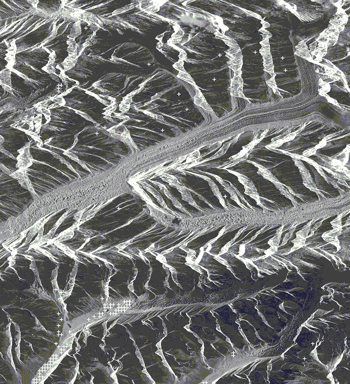
A second run with

offset_pwr <SLC-1> <SLC-2> <SLC1_par> <SLC2_par> <OFF_par> <offs> <snr> 64 64 - 4 128 128 7.0 0
offset_fit <offs> <snr> <OFF_par> [coffs] [coffsets] 15.0 4 1

gave me:

Now I am satisfied! :D